eBPF and Perfetto UI proved me wrong

Table of contents [show/hide]

This blog post is about an experience of debugging MMTk using a tracing and visualisation tool based on eBPF and Perfetto UI. During debugging, I tried to guess what went wrong for many times, but the tool showed what actually happened and proved me wrong each time.

The anomaly

I made a pull request for MMTk-core. It sped up all benchmarks in the DaCapo Benchmarks suite, except the jython benchmark which became 3x slower in stop-the-world (STW) time (i.e. time spent doing garbage collection).

In the following plot, build3 is the baseline revision, build1 is an intermediate commit, and build2 contains my final change. The time is normalised to build3 for each benchmark.

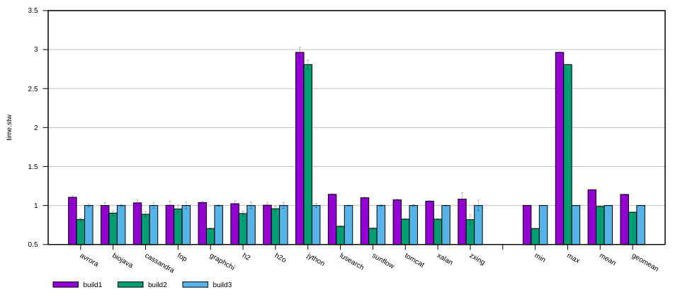
I could conclude that the jython benchmark had some abnormal behaviour and the overall result (build2 in geomean) was still speeding up. But the 3x slow-down was too significant to overlook. I decided to investigate.

eBPF-based tracing and visualisation

Strangely, the slow-down was only observable on two of the testing machines in our laboratory. When I re-ran the jython benchmark with build1, build2 and build3 on my laptop, their stop-the-world (STW) times were similar. They were either equally good or equally bad. I guessed they were equally bad. I inferred that the problem was non-deterministic. It may be triggered under some unknown conditions.

The slow-down was in the STW time, which meant some GC activities became slower. But how would I know which GC activity was slow?

At that time, my colleagues were developing a eBPF-based tracing tool which can record the duration of each work packet during a GC, and visualise them on a timeline. Its overhead when not used was so low that we can leave the trace points in the code in release builds, and active them whenever we want to measure something. I thought it was the perfect tool for my task. Although the tool was still being developed, I asked my colleagues for a copy and gave it a try anyway.

The tool included a patch to the MMTk Core source code which inserted USDT (user statically-defined tracing) tracepoints at important places. They were compiled as NOP instructions, but could be patched at run time to execute custom code. I used the bpftrace command line utility to activate those tracepoints to record the start and the end of each work packet, then used a script to format the output into a JSON format which was then sent to Perfetto UI. Perfetto UI showed what happened during a GC in a timeline.

Actually, I observed two different timeline patterns from different GCs when running the jython benchmark.

The first pattern (I called it the ‘kind 1’ GC) looked like this:

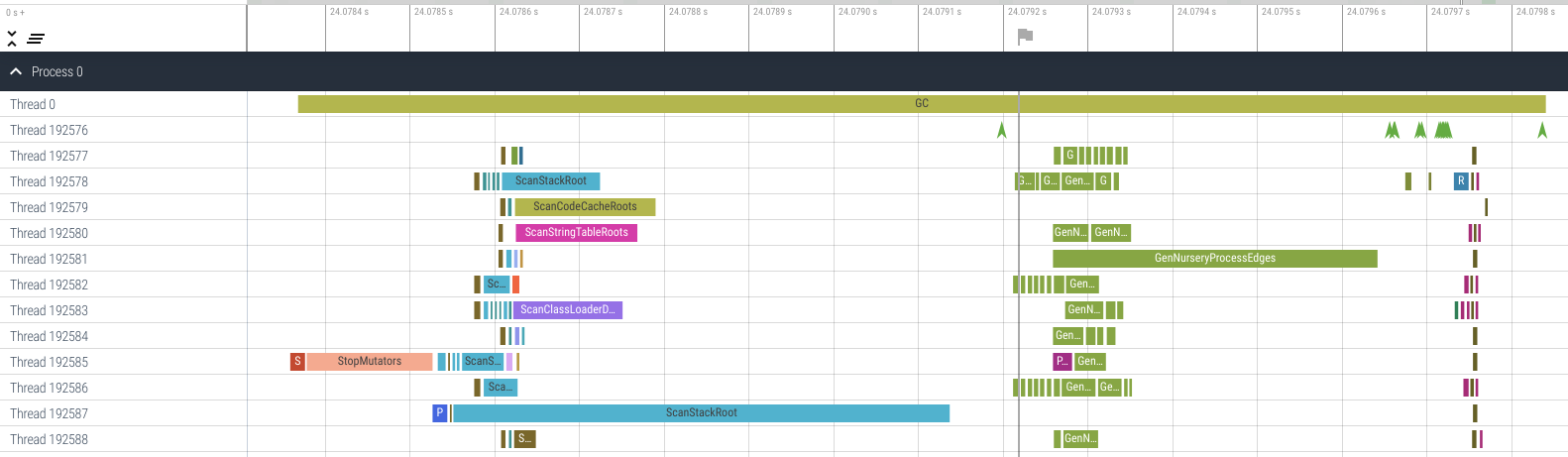
This was a minor GC in a generational GC algorithm, and it was quite a typical one.

The green arrows in Thread 192576 marked the start of each stage.

• The Prepare stage happened before the green arrow near the ‘24.0792 s’ mark, during which there were many work packets named ScanXxxxRoot(s).
• The Closure stage happened between that green arrow and the next green arrow after the ‘24.0796 s’ mark, during which there were many green GenNurseryProcessEdges work packets.
• Then there were some short intermediate stages, such as FinalRefClosure which handled finalization.
• The Release stage happened near the end of the GC between the ‘24.0797 s’ and the ‘24.0798 s’ marks, where each worker executed some clean-up job.

Since a minor GC does not trace much objects (it only traces the nursery), the Closure stage did not took much time. A ‘kind 1’ GC typically takes only about 1 ms, despite the ScanStackRoot work packet in Thread 192587 and the GenNurseryProcessEdges packet in Thread 192581 being a bit too big due to an unrelated load-imbalance problem.

The second pattern (I called it the ‘kind 2’ GC) looked like this:

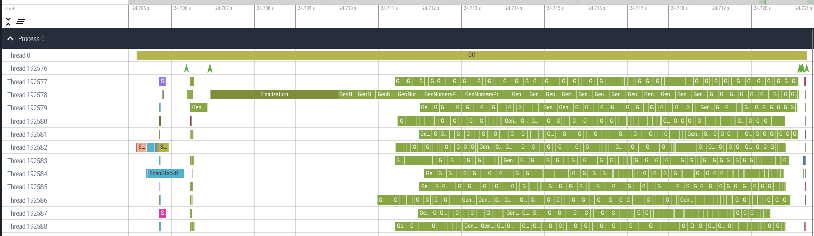
This was also a minor (nursery) GC, too, seen form packet name GenNurseryProcessEdges. The Prepare stage and the Closure stage are similar to the ‘kind 1’. (Please note the horizontal scale of the timeline. The Prepare and the Closure stages were in the far left of this plot, before the Finalization packet.) What was interesting was the FinalRefClosure stage where finalization were done. After the Finalization packet, lots of GenNurseryProcessEdges work packets were executed. It was obvious that finalization resurrected many objects. A ‘kind 2’ GC is significantly longer than a ‘kind 1’ GC. It may take more than 15 ms to execute.

Given that finalization is non-deterministic, we might infer that the slow-down was caused by an excessive amount of finalization due to non-deterministic execution. Problem solved…, or was it? I still needed to verify.

Printing out the GC times

I printed out the GC time of each GC in jython when running on a test machine in the lab.

With 1500M heap size, the GC time (i.e. STW time) of the original code (build3) and my modification (build2) were:

• Before: 2,2,1,8,1,2,9ms
• After: 1,21,1,10,1,20,9ms

So the GCs that took 21, 10, 20 and 9 ms should be doing finalization, right?

I ran it on another test machine (with identical hardware) with 1500M heap, too:

• Before: 2,1,1,11,1,3,8ms
• After: 2,27,1,9,2,25,8ms

The results were similar between two machines. I then tried to reduce the heap size.

When I reduce the heap size to 500M:

• Before: 1,1,1,1,1,2,2,1,1,5,9,2,2,1,2,1,1,2,1,2,1,5,8,4
• After: 1,1,1,1,1,30,1,1,1,4,8,1,1,1,1,1,1,27,1,1,1,3,8,4

When I reduce the heap size to 250M:

• Before: 1,1,2,2,2,1,1,2,1,1,2,1,3,1,2,2,1,1,1,1,2,4,5,6,4,1,1,2,1,1,2,1,1,1,2,2,1,2,2,2,2,2,1,1,1,1,1,2,1,1,4,7,5,4,2,2,
• After: 1,1,1,1,1,1,1,1,1,1,2,1,29,1,1,1,2,1,1,1,1,4,6,6,1,2,1,1,1,1,1,1,1,1,1,1,1,1,1,2,25,1,1,1,1,1,1,1,1,1,4,5,5,4,1,1,

If the slow-down were caused by excessive finalization, I would expect one build to have more GCs that had more than 15 ms of STW time. But it was not the case. Two builds had the same number of GCs, and the GC time of each pair of corresponding GCs were similar, too, except two pairs. No matter how large the heap size was, there were always exactly two GCs that took more than 20 ms in the ‘After’ case (i.e. build2, the build with my PR applied). For other GCs, most of them took 1 ms and I assumed they were the ‘kind 1’ GCs; some of them took 5 ms to 10 ms and I guessed they were the ‘kind 2’ GCs.

So the two 20+ ms GCs were interesting. What happened during them? Were they slow because of finalization, too?

I re-ran the test at 250M heap size on my laptop. Strange things happened.

• Before: 1,1,1,1,1,2,1,1,1,1,1,2,1,2,2,1,2,2,2,2,1,2,1,5,7,7,6,1,2,1,1,1,2,1,1,1,2,1,2,2,2,1,1,2,2,2,1,2,2,2,1,1,2,2,2,1,5,7,6,5,1,2,2,
• After: 2,1,1,1,1,1,1,1,2,1,1,1,2,2,2,1,2,2,2,2,1,1,1,7,8,7,5,1,1,2,1,1,1,1,1,1,2,2,1,1,1,2,1,2,2,2,1,1,1,1,1,1,1,1,1,4,6,6,6,4,1,1,

The mysterious 20 ms GCs vanished!

This meant those 20 ms GCs were definitely not ‘kind 2’ GCs because otherwise I would have observed them on my laptop.

This also meant I could not capture those mysterious 20 ms GCs on my laptop using eBPF tracing. I could only capture them on the lab machines.

Manual tracing

Since I could not use eBPF tracing on the lab machine due to lack of root access, I manually instrumented the code to log the starts and ends of each work packets. I printed the log in the same format as the output of the eBPF tool, used the same script to process the log into the JSON format, and fed the JSON into Perfetto UI. Then a nice timeline came out. (And you can try it by your self. Load this log file into https://www.ui.perfetto.dev/ and browse the timeline interactively.)

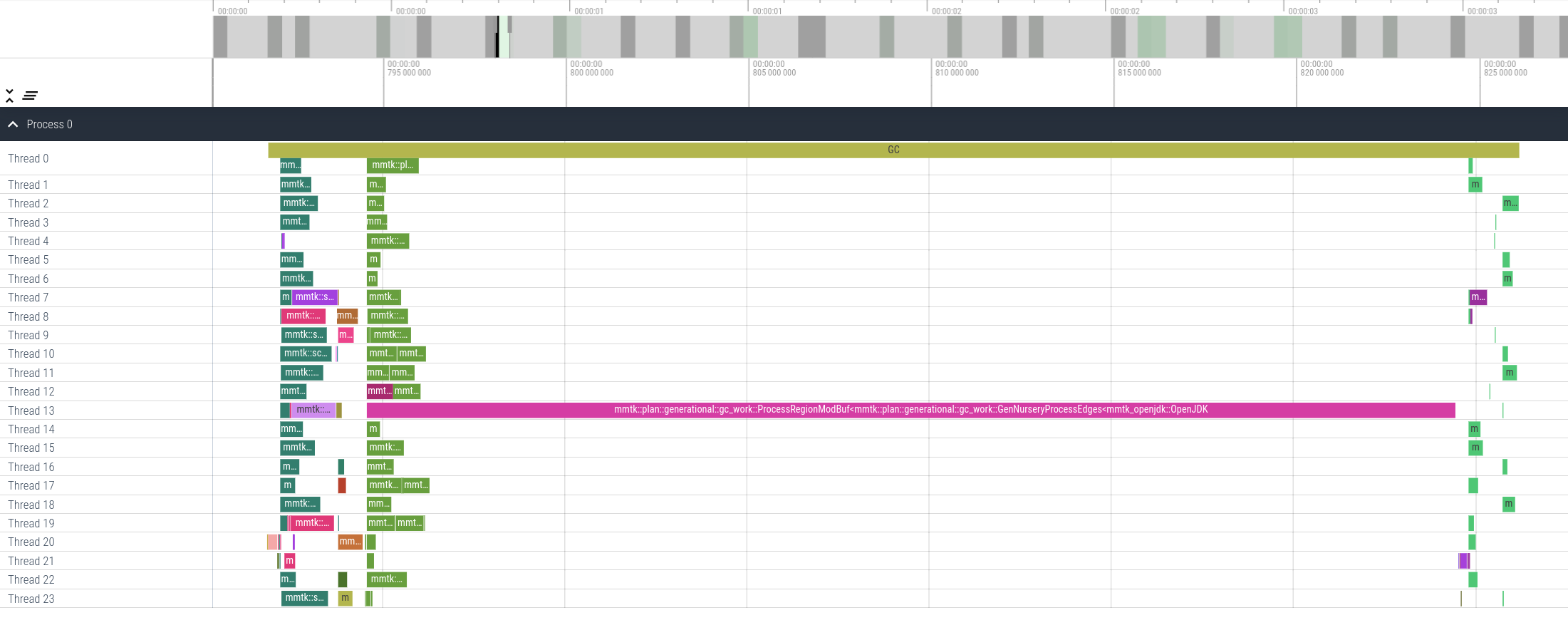
And that was a strange timeline, too. Why was the ProcessRegionModBuf work packet so large? The purpose of the ProcessRegionModBuf work packet is handling the write barriers for bulk accesses of arrays (such as System.arraycopy() in Java) between the last GC and this GC.

There might be two possibilities:

1. The jython benchmark did call System.arraycopy() on a very large array, therefore the work packet should exist in order to process the write barrier. However, it did not appear in the ‘Before’ build (build3) due to a bug.
2. The jython benchmark did not copy large arrays at all, but a bug (probably introduced or triggered by my PR) caused the write barrier to erroneously record an access to a large array while it did not, resulting in an abnormally large ProcessRegionModBuf work packet.

So which one was true?

Hacking the write barriers

I added a log at the place where a ProcessRegionModBuf work packet is created in order to see the sizes of the ProcessRegionModBuf work packets.

When running on the lab machines,

• in the ‘before’ build, all ProcessRegionModBuf work packets had lengths of 0;
• in the ‘after’ build, ProcessRegionModBuf came in all different sizes.

When running on my laptop, all ProcessRegionModBuf work packets had lengths of 0.

But it does not make sense to copy zero elements using System.arraycopy()!

Then I had reasons to believe that there was a bug in the write barrier code so that in the ‘before’ build, the write barrier failed to record any accessed array regions, making the GC erroneously faster than it should have been. In the ‘after’ build, the bug was not triggered, so the accessed array regions were recorded by write barriers as usual, resulting in a longer but actually normal STW time. In other words, it was not my PR that made the STW time longer, but the STW time had been shorter than it should have been.

One of my colleagues reminded me that there was an un-merged commit that fixes a bug in the write barrier code in the MMTK-OpenJDK binding. It was intended to fix an unrelated bug, but it was still worth giving it a try.

I cherry-picked that commit, and… Voila! It fixed the bug! The ‘before’ build then exhibited the two 20+ ms GCs, just like the ‘after’ build.

• Before: 1,2,2,1,1,29,1,1,2,5,8,2,1,1,1,2,1,29,1,1,1,4,9,3,

Conclusion

At this point, we could draw the conclusion. The STW time for the jython benchmark should have been 3x longer. However, due to the bug fixed by this commit, the barrier did not record the bulk accesses to arrays properly, and therefore did less things than it should have done. When I was running the DaCapo benchmarks at the beginning of this blog post, I set the heap size too large (1500M). With such a large heap size, GC was only triggered a few times, and the proportion of write barrier handling became more significant in STW time. Therefore the STW time for jython was only 1/3 of the normal time due to the missing write barrier handling.

However, my PR changed the behaviour in some way, and the bug was somehow not triggered when running on the test machines in the lab. And the sub-optimal implementation of the ProcessRegionModBuf work packet stuffed all the array slices delivered from barriers into one single vector, making it impossible to parallelise. It gave us a false impression that my PR made the jython benchmark 3x slower on the lab machines.

And due to non-determinism, the bug was still reproducible on my laptop with my PR applied. That was why I saw the 3x slow-down on the lab machines but not on my laptop.

What did I learn?

There is a saying that ‘One can not optimise things that one can not measure’. It is very true. I can hypothesise what caused the performance problem, but I can never be sure unless I verify it with experiment. In this example, I first thought the slow-down was just some random behaviour of the jython benchmark. I then thought the slow-down was due to excessive finalization. But experiments showed that the actual cause was a bug in the write barrier.

And the visualisation tool is a very useful one. It first showed me that some GCs took longer time due to finalisation, and it then showed me that there were even longer GCs due to buggy and sub-optimal write barrier handling. It is such a useful tool because with the timeline in front of me, I no longer need to guess what slowed things down. I just look at the timeline, and the work packet that becomes the bottleneck will stand out of the crowd. Since the eBPF-based tracing and visualisation tool was created, I have been using it to debug many performance issues in GC, including the execution of obj_free, various weak table processing tasks, and the load-balancing problems in the MMTk-Ruby binding.

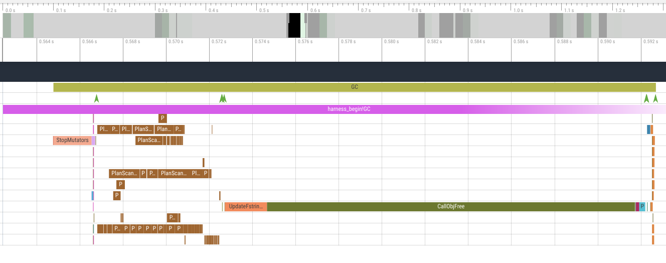
For example, when I saw the following timeline, I knew the handling of obj_free was the bottleneck.

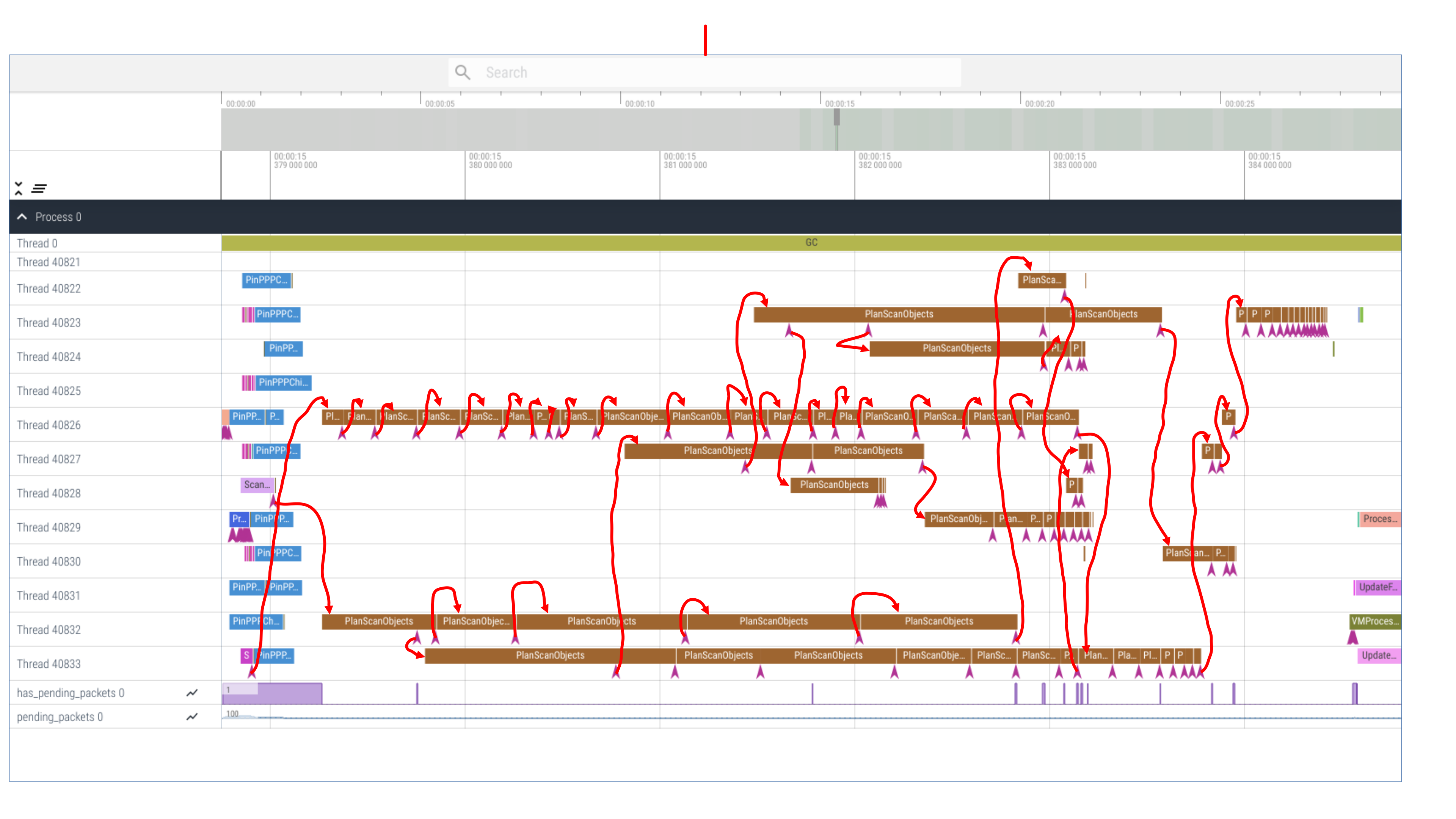
When I saw the following timeline (with manual annotation of which work packet created which), I knew the load balancing of the transitive closure stage needed to be improved.

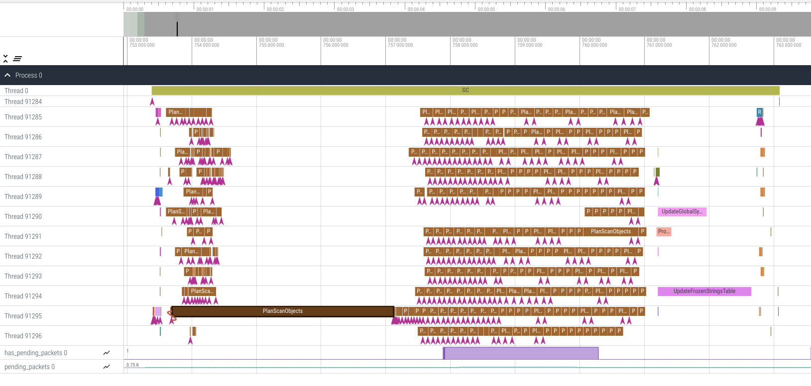
And when I saw the following timeline, I knew the general load balancing was improved, but some objects took significantly longer to scan than other objects, and I should focus on those objects because they were the bottleneck.

The tool

I thank Claire Huang, Zixian Cai, and Prof. Steve Blackburn for creating such a useful tool.

The tool is now publicly available. The code has been merged into the master branch of mmtk-core. Related tools and documentation can be found in this directory.

The paper that describes this work is freely available online under the Creative Commons Attribution 4.0 International License, and will be presented in the MPLR 2023 conference.